
Loan analysts use Excel nearly every day. Many learned the formulas, functions, and how to set up spreads on their own, asking colleagues or searching the internet for help. Even with their hands-on skills, there are times when there are Excel formulas financial analysts want to use, but they aren’t sure how to apply them to the specific situation. The analyst ends up wasting a lot of time searching for the answer, time that could be better spent elsewhere.
Sound familiar? What you need is a little guidance without having to search forever online to find it.
Essential Excel Formulas You Can Start Using Today
Our Support Team has a broad range of experience, from banking and credit to data analysis, and our product designers also have Excel experience. When we designed FISCAL Forward software, we wanted it to be easy to use out of the box and similar to tools loan analysts are already familiar with. While we specialize in spreading and tracking software, we also know a thing or two about Excel spreadsheets.
To help you advance your Excel skills, we’ve compiled a list of essential Excel formulas and functions we’ve found especially helpful in analyzing small business loans.
SUM
This fairly easy formula is often the first one people learn. It adds values in various cells either for a sequence of cells, such as:
=SUM(A2:A10) adds the values in cells A2 through A10.
Or separate sets of cells in the spreadsheet, such as:
=SUM(A2:A10, C2:C10) adds the values in cells A2:10, as well as cells C2:C10, then adds those totals together.
While this may seem elementary to some, we still see many spreadsheets that contain formulas like:
=A2 + A3 + A4 + A5...
The problem with this approach is that if a user subsequently inserts a Row within the range, it will not be included in the formula, but a SUM formula will update automatically to include the new row.
ABS
Most of the time, numbers entered into a spreadsheet will be predictably positive or negative, but in some cases, you won’t know how the user will choose to enter a value. This is where using an absolute value, that is, the number without the positive or negative attribute indicated, can save the day. This is done with the formula:
ABS(number) Or ABS(cell)
For example ABS(-2) = 2
Or, if cell A2 contains the value -4 then ABS(A2) = 4
Similarly, if cell A2 contains the value 4 then ABS(A2) = 4
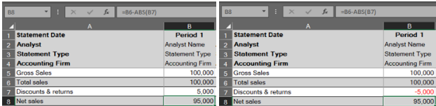
A common use case for this would be Discounts and Returns, which are deducted from Gross Sales to determine Net Sales. Because Discounts and Returns are generally reported at a negative value on financial statements and tax returns, it would be normal to use a simple addition or SUM formula, which would add the positive Sales to the negative Discounts/Returns, resulting in an accurate Net Sales.
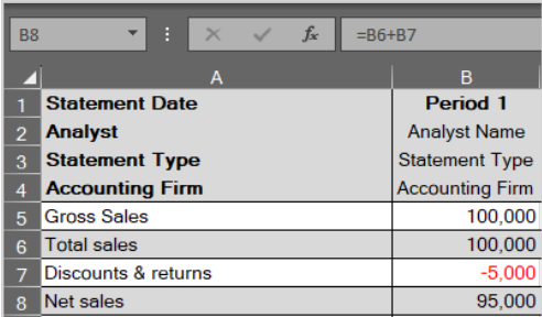
You might also assume the user would enter the value as a positive, and use =B6 - B7.
However, if the user enters Discounts and Returns opposite of your expectation (whether positive or negative), the above approaches would increase Gross Sales by the amount of Discounts/Returns, rather than decreasing it.
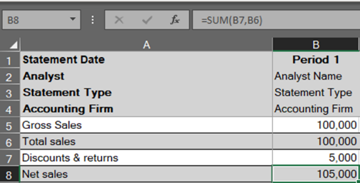
By introducing an ABS() formula into the reference to Discounts and Returns, we can ensure the value comes out correctly regardless of user input:
IF
The IF function lets you make logical comparisons between a value and what you expect, yielding one of two results. The first is if your comparison is True, while the second is if your comparison is False.
For example, =IF(C2=”Yes”,1,2) says IF(C2 = Yes, then return a 1, otherwise return a 2).
This can be used with numbers and text. For example, to document whether something is within or over budget, insert the IF formula:
IF(C2 Is Greater Than B2, then return “Over Budget”, otherwise return “Within Budget”)
IF statements can be used for all kinds of things, but formatting is a common one. For instance, when calculating a Profit Margin, Common Size value, or Year to Year change, a formula could return a #DIV/0 error, indicating that you are dividing by zero.
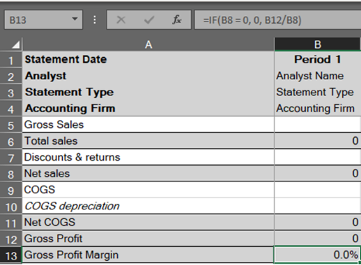
By controlling for this problem with an IF statement: =IF(B8 = 0, 0, B12 / B8), we can remove this error:
ROUND
The ROUND function in Excel rounds a decimal number to a specified number of digits. If cell A1 contains 23.7825, for example, and you want to round that value to two decimal places, use the formula:
=ROUND(A1, 2)
The result is 23.78 in cell A1.
While this can be accomplished visually using Format Cells, the underlying value would not be rounded, so the raw value would be used in subsequent formulas and calculations.
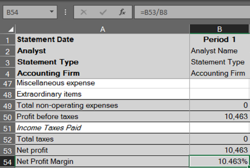
As with the other examples above, ROUND() can be used with other formulas, like in the Net Profit Margin calculation below:
Unrounded:
Rounded (additional decimals left visible to show the value has been rounded):
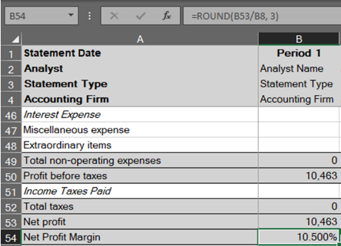
This is another basic formula that is easy to introduce into your existing financial statement spreading templates to improve formatting and consistency.
VLOOKUP
VLOOKUP is the most advanced formula we will look at in this post–and certainly, the most difficult to implement effectively–but it is also the most powerful when used correctly. What is VLOOKUP? It helps you find a specific value, related to another value, in a specific location using these parameters:
- What you want to look up.
- Where you want to look for it.
- The column number in the range containing the value to return.
- Return an approximate or exact match – indicated as 1/TRUE, or 0/FALSE.
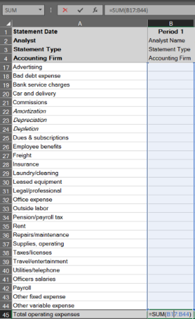
To use VLOOKUP, to locate a certain expense, you can set up a formula like this:
=VLOOKUP(“Marketing”,[array],2,FALSE)+VLOOKUP(“Rent”,[array],2,FALSE)+etc
Continue this formula with the names of expense items you’d like to add for a total you’re sure is associated with those expenses, even if you add or delete rows or list those expenses somewhere other than their original location.
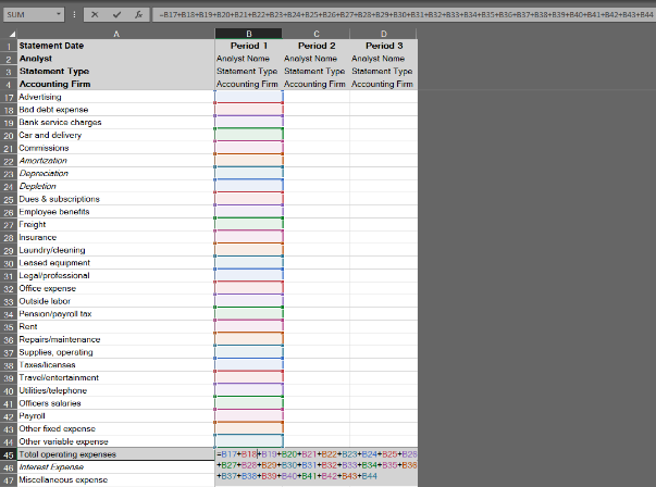
As an example, when calculating EBITDA, it would be common to pre-define rows for Interest, Taxes, Depreciation, Amortization, etc. add back expenses, and expect the user to enter those expenses in the defined row. The formula for EBITDA then might look something like this:
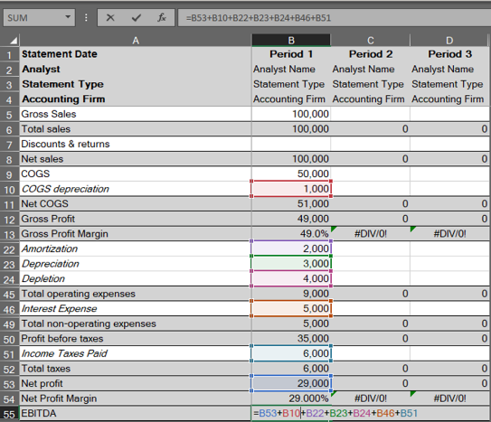
The problem with this approach is that the user may choose to change Row 22 to “Advertising” and subsequently put Amortization on another row. If using the formula above, the Advertising expense would then be added back as part of EBITDA, rather than Amortization, unless you manually edit the formula to account for the change.
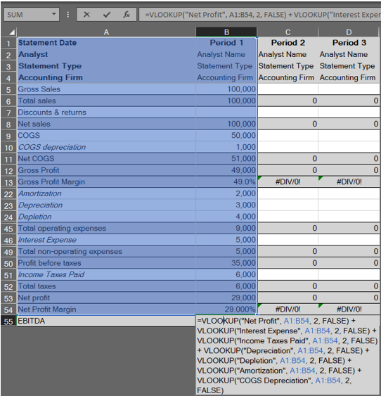
Using VLOOKUP instead of simple cell selection in your formulas can ensure that the correct accounts are captured regardless of their location in the spreadsheet:
Excel Formula Use Cases
Now that we’ve covered the essential formulas, let’s explore how they’re used in more complex cases.
Global Cash Flow
While the formula for Global Cash Flow is itself relatively straightforward, if you want to eliminate duplicate data entry and instead have the various components flow automatically into your calculations, it can become complex quite quickly. Depending on how many business entities and personal guarantors are involved in a deal, you may need to reference multiple values in a variety of worksheets.
This is where you can combine the powerful VLOOKUP functionality with Sheet references to pull in values across an entire workbook. You can do this by creating the following formula in the EBITDA cell:
=VLOOKUP(“EBITDA”,'[SheetName]'![array],2,FALSE)
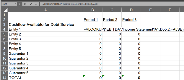
The result? No matter how many changes the user makes to the input worksheets, the formula will locate the row description “EBITDA” and return the value in the second (or third, fourth, etc.) column over from it. By ensuring you’re always drawing the value from the cell related to” EBITDA”, you can be certain you’re using the correct data for the formula, and eliminate the need to re-key it multiple times.
For a step-by-step guide to setting up Global Cash Flow, read our post, “Global Cash Flow Analysis: How to Get it Right.”

Debt Service Coverage Ratio (DSCR)
The Debt Service Coverage Ratio shows the number of times a business’s cash flow available for debt service can cover its debt payments in a given year.
The formula for DSCR is: DSCR = Cashflow Available for Debt Service / Total Debt Service; like the Global Cash Flow above, the formula itself is very straightforward, but being sure you’re using the correct values after unpredictable end-user changes is much more complicated.
This is another place where VLOOKUP formulas come in handy, pulling important numbers from cash flow available for debt service (CFADS)- such as Net Profit, Interest Expense, Taxes, and others- dividends and distributions given to owners, etc. As noted in the VLOOKUP section above, using VLOOKUP in your formula can provide consistent results regardless of user input:

To get more expert tips on how to more accurately calculate DSCR, read our blog post, “How to Quickly Calculate Debt Service Coverage Ratio [Guide for Banks]”
Mastering Loan Underwriting Formulas Beyond Excel
While these formulas and functions will save you time, small banks and credit unions can exponentially improve their efficiency and accuracy with spreading software. With unbreakable templates and automation features, loan analysts will save countless hours currently spent building and reviewing Excel spreadsheets.
As mentioned above, we have extensive experience in formulas for financial analysts, both in Excel and in our software solutions. Want to know more about how we can help? Our team is happy to talk to you.